第四章 噪音 | Noise
在英文中,noise (噪音)指的是不想要的或是令人不悅的聲音。在訊號處理的領域裡,它有兩個不同的意思:- 如同英文的意思,它意指不想要的訊號。如果兩個訊號互相干擾,彼此都會認為是噪音。
- 噪音也可以被認為是有許多頻率成份的訊號,所以它沒有諧波結構。我們在前幾章的週期訊號會有諧波結構。
這章的程式碼在 chap04.ipynb。要找到它請看 0.2 節。你也可以到 http://tinyurl.com/thinkdsp04 查看。
4.1 不相關噪音 | Uncorrelated noise
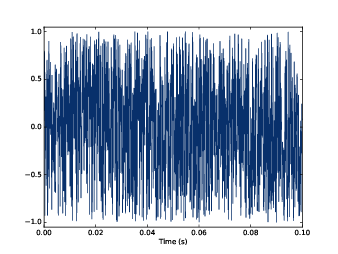
圖4.1:不相關均勻噪音的波形
最簡單來瞭解噪音的方式就是製造它,最容易製造的噪音就是「不相關均勻噪音 uncorrelated uniform noise (UU noise)」。Uniform 均勻,指的是訊號的值是均勻分佈的隨機值,也就是在範圍中的每個值出現機率都一樣。uncorrelated 不相關,指的是每個值都獨立,不互相影響。也就是知道一個值之後,也沒有訊息可以預測其他的值。
UU noise 的程式碼如下:
class UncorrelatedUniformNoise(_Noise):

    def evaluate(self, ts):
        ys = np.random.uniform(-self.amp, self.amp, len(ts))
        return ys
照舊,evaluate 依照 ts 來計算對應的訊號值 ys。它使用 np.random.uniform,這是從均勻分佈產生值的函式。在這個例子裡,數值範圍從 -amp 到 amp。
接下來的例子是產生一個 UU noise,持續時間 0.5 秒,取樣率每秒 11025 次。
signal = thinkdsp.UncorrelatedUniformNoise()
wave = signal.make_wave(duration=0.5, framerate=11025)
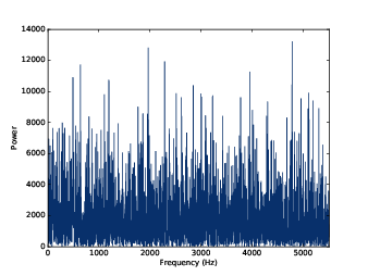
圖4.2:不相關均勻噪音的能量頻譜
現在來看看它的頻譜:
spectrum = wave.make_spectrum()
spectrum.plot_power()
圖4.2 顯示了結果,跟訊號的波形相同,頻譜也看起來很隨機。事實上,隨機這個字必須更精確定義。在噪音訊號或頻譜這方面,至少有三件事要知道:
- 分佈:隨機訊號的分佈由一組可能的值與裡面的值出現的機率所組成。例如,在均勻噪音的訊號,值的範圍是從 -1 到 1,所有的值出現的機率都相同。另外一種分佈是高斯噪音,值的範圍是負無窮大到正無窮大,但是接近 0 的值有比較高的出現機率,兩端下降的機率則依照高斯曲線(或說鐘形曲線)
- 相關性:在訊號中的每個值是否獨立於其他的值,或是它們彼此相依?在 UU noise,值是獨立的。另一個相關性的例子是布朗噪音,每個值,都是前一個值的總和再加上隨機的一個步進值。所以如果訊號的值在某個特定點是高的,我們可以預期它接下來還是高的,如果原來是低的,也會預期它會留在低處。
- 功率與頻率的關係:在 UU noise 的頻譜裡,每個頻率的功率是與分佈相同。也就是說平均功率對於所有頻率來說是一樣的。與之不同的一個例子是 pink noise,它的功率與頻率有相反的關係,也就是在頻率 f 的功率會正比於 1/f。
4.2 積分頻譜 | Integrated spectrum
對於 UU noise 來說,使用積分頻譜,我們可以比較清楚看到功率與頻率的關係。積分頻譜會是頻率的函數,隨著頻率增加而顯示到某頻率的功率的累積和。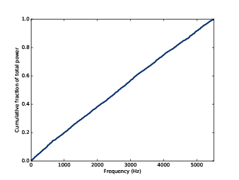
圖4.3:不相關均勻噪音的積分頻譜
Spectrum 提供了一個方法計算積分頻譜 IntegratedSpectrum:
def make_integrated_spectrum(self):
    cs = np.cumsum(self.power)
    cs /= cs[-1]
    return IntegratedSpectrum(cs, self.fs)
回傳的是 IntegratedSpectrum,這是類別的定義:
class IntegratedSpectrum(object):
    def __init__(self, cs, fs):
        self.cs = cs
        self.fs = fs
integ = spectrum.make_integrated_spectrum()
integ.plot_power()
4.3 布朗噪音 | Brownian noise
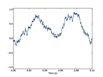
圖4.4:布朗噪音的波形
UU noise 說是不相關,是指它的每個值都與其他值無關。一個有相關的例子是「布朗噪音 Brownian noise」,裡面的每個值都是前值的總和再加一個隨機步進值。
會叫做布朗,是類比於布朗運動。國中應該學過,一個微粒在液體裡看起來像是隨機的運動,因為它被液體裡看不見的作用而影響。布朗運動常用「隨機行走 random walk」來描述,這是一個路徑的數學模型,步進值是隨機分佈。
以一維的隨機行走來說,微粒在每個時間只能往上或往下,微粒的位置,就是前面幾步的總和。
這個觀察提供了一個產生布朗噪音的方法,產生不相關隨機的步進值,然後把它們加起來。所以底下的程式碼是這樣寫的:
class BrownianNoise(_Noise):

    def evaluate(self, ts):
        dys = np.random.uniform(-1, 1, len(ts))
        ys = np.cumsum(dys)
        ys = normalize(unbias(ys), self.amp)
        return ys
因為加總會讓值離開 -1 到 1 範圍,所以需要 unbias 讓平均值移動到 0,最後 normalize 調整上下值到想要的最大振幅的值。
要產生 BrownianNoise 物件且畫一個波形,程式碼如下:
signal = thinkdsp.BrownianNoise()
wave = signal.make_wave(duration=0.5, framerate=11025)
wave.plot()
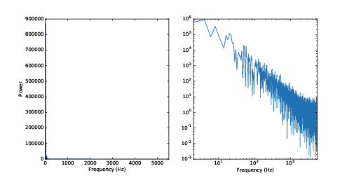
圖4.5:布朗噪音的頻譜畫在線性座標圖與 log-log 對數座標圖上
如果你畫了布朗噪音的頻譜放在線性座標圖上,像圖4.5 左圖。幾乎功率都在低頻,若用線性座標畫,高頻部份幾乎看不到。
為了要看清楚頻譜的形狀,我們可以把功率密度與頻率畫在 log-log 比例,也就是對數座標圖上:
spectrum = wave.make_spectrum()
spectrum.plot_power(low=1, linewidth=1, alpha=0.5)
thinkplot.config(xscale='log', yscale='log')
Spectrum 提供 estimate_slope 方法,它使用 scipy 計算最小平方差來擬合(fit)功率頻譜:
#class Spectrum

    def estimate_slope(self):
        x = np.log(self.fs[1:])
        y = np.log(self.power[1:])
        t = scipy.stats.linregress(x,y)
        return t
estimate 回傳 scipy.stats.linegress 的結果,它是一個物件,包含了斜率與截距的估計值、判定係數(coefficient of determination )、p-值、標準差。在這裡我們只需要斜率。
對布朗噪音來說,功率頻譜的斜率大約是 -2 (第九章會知道為什麼)。所以我們可以寫下這個關係式:
是功率, 是頻率, 是直線的截距,它現在對我們來說不重要。兩邊都取指數,會得到:
是 ,這裡我們還是先不討論它。重要的是,功率與 成正比,這是布朗噪音的特徵。
布朗噪音也叫做紅噪音,與白噪音一樣的原因。如果把可見光依照功率正比於的關係組合起來,多數功率會出現在頻譜的低頻位置,那是紅光。布朗噪音在英文也有人寫成 “brown noise”,我想這會讓人誤會,所以就不這樣寫。
4.4 粉紅噪音 | Pink Noise
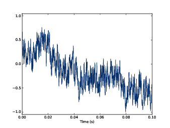
圖4.6:β=1 的 pink noise 的波形
紅噪音的頻率與功率的關係式是
這個指數 2 沒有什麼特別。那讓我們改成比較通用的寫法,讓我們可以用任意的指數值 β 產生噪音:
在 β = 0 的時候,對於所有的頻率來說,功率是常數,產生的就是白噪音。當 β = 2 的時候,產生的是紅噪音。
那麼,β 在 0 跟 2 之間呢?產生的是白與紅之間的噪音,所以叫做「pink noise 粉紅噪音」
有幾個方法可以產生粉紅噪音,最簡單是產生白噪音,然後用個低通過濾器,濾出想要的成份。thinkdsp 提供一個類別:
class PinkNoise(_Noise):

    def __init__(self, amp=1.0, beta=1.0):
        self.amp = amp
        self.beta = beta
def make_wave(self, duration=1, start=0, framerate=11025):
    signal = UncorrelatedUniformNoise()
    wave = signal.make_wave(duration, start, framerate)
    spectrum = wave.make_spectrum()

    spectrum.pink_filter(beta=self.beta)

    wave2 = spectrum.make_wave()
    wave2.unbias()
    wave2.normalize(self.amp)
    return wave2
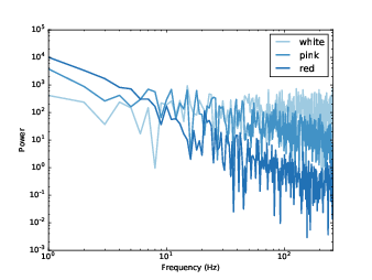
圖4.7:白、粉紅、紅噪音的頻譜,畫在 log-log 對數座標上
make_wave 產生白噪音的波,計算它的頻譜,設定好過濾器的指數值,執行過濾的動作。然後再從頻譜轉回波,然後調整偏置與正規化到想要的振幅。
Spectrum 提供的 pink_filter 如下:
def pink_filter(self, beta=1.0):
    denom = self.fs ** (beta/2.0)
    denom[0] = 1
    self.hs /= denom
圖4.6 顯示最後的結果,跟布朗噪音一樣,它也是忽上忽下與前值有相關,但它看起來又比較隨機。在下一章,我們會回頭再觀察它,屆時會更精確地說明相關性與隨機。
最後,圖4.7 顯示白、粉紅、紅噪音在同一張對數圖上,指數 β 與圖上的斜率的關係也顯示在圖上。
4.5 高斯噪音 | Gaussian noise
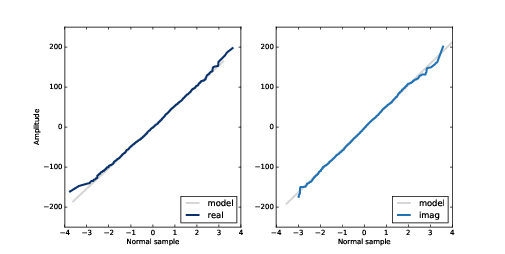
圖4.8:常態機率圖:高斯噪音的頻譜的實部與虛部
我們開始時是介紹 UU noise (不相關均勻噪音),並且說明 UU noise 之所以叫白噪音是因為從頻譜來看,每個頻率的功率是一樣的。
但當人們談到白噪音,不見得都是 UU noise。事實上,他們更常指的是所謂的「不相關高斯噪音 uncorrelated Gaussian(UG) Noise」。
thinkdsp 提供 UG noise 的實作:
class UncorrelatedGaussianNoise(_Noise):

    def evaluate(self, ts):
        ys = np.random.normal(0, self.amp, len(ts))
        return ys
UG noise 在很多地方跟 UU noise 很像。在頻譜上,每個頻率的功率平均來說是相同的,所以 UG 也是白的。它還有另一個有趣的性質,UG noise 的頻譜也是 UG noise。更精確地說,頻譜的實部與虛部也是不相關高斯值。
為測試這個宣告,我們可以產生 UG noise 的頻譜,然後產生 “normal probability plot”(常態機率圖)。用這種圖形化方式來驗證是否一個分佈是高斯分佈。
signal = thinkdsp.UncorrelatedGaussianNoise()
wave = signal.make_wave(duration=0.5, framerate=11025)
spectrum = wave.make_spectrum()

thinkstats2.NormalProbabilityPlot(spectrum.real)
thinkstats2.NormalProbabilityPlot(spectrum.imag)
圖4.8 顯示了結果,灰線顯示由資料擬合成一個直線模型,而深色線顯示資料。
在常態機率圖裡,一條直線表示資料來自高斯分佈。除了一些隨機變化的情況,這些直線滿直的,這表示 UG noise 的頻譜是 UG noise。
UU noise 的頻譜也是 UG noise,至少是相近。事實上,依據中央極限原理,大多數的不相關噪音的頻譜,都近似高斯分佈,只要分佈有有限的平均值與標準差,而且取樣數目夠大。
4.6 練習
Solutions to these exercises are in chap04soln.ipynb.Exercise 1 “A Soft Murmur” is a web site that plays a mixture of natural noise sources, including rain, waves, wind, etc. At http://asoftmurmur.com/about/ you can find their list of recordings, most of which are at http://freesound.org.
Download a few of these files and compute the spectrum of each signal. Does the power spectrum look like white noise, pink noise, or Brownian noise? How does the spectrum vary over time?
Exercise 2 In a noise signal, the mixture of frequencies changes over time. In the long run, we expect the power at all frequencies to be equal, but in any sample, the power at each frequency is random.
To estimate the long-term average power at each frequency, we can break a long signal into segments, compute the power spectrum for each segment, and then compute the average across the segments. You can read more about this algorithm at http://en.wikipedia.org/wiki/Bartlett‘s_method.
Implement Bartlett’s method and use it to estimate the power spectrum for a noise wave. Hint: look at the implementation of make_spectrogram.
Exercise 3 At http://www.coindesk.com you can download the daily price of a BitCoin as a CSV file. Read this file and compute the spectrum of BitCoin prices as a function of time. Does it resemble white, pink, or Brownian noise?
Exercise 4 A Geiger counter is a device that detects radiation. When an ionizing particle strikes the detector, it outputs a surge of current. The total output at a point in time can be modeled as uncorrelated Poisson (UP) noise, where each sample is a random quantity from a Poisson distribution, which corresponds to the number of particles detected during an interval.
Write a class called UncorrelatedPoissonNoise that inherits from thinkdsp._Noise and provides evaluate. It should use np.random.poisson to generate random values from a Poisson distribution. The parameter of this function, lam, is the average number of particles during each interval. You can use the attribute amp to specify lam. For example, if the frame rate is 10 kHz and amp is 0.001, we expect about 10 “clicks” per second.
Generate about a second of UP noise and listen to it. For low values of amp, like 0.001, it should sound like a Geiger counter. For higher values it should sound like white noise. Compute and plot the power spectrum to see whether it looks like white noise.
Exercise 5 The algorithm in this chapter for generating pink noise is conceptually simple but computationally expensive. There are more efficient alternatives, like the Voss-McCartney algorithm. Research this method, implement it, compute the spectrum of the result, and confirm that it has the desired relationship between power and frequency.


沒有留言:
張貼留言