第九章 微分與積分 | Differentiation and Integration
這一章是前章的補遺,在探討時間域的 window 與頻率域的濾波器。我們會特別來探討 finite difference window 的影響。它是近似的差異累積加總的操作,其效果接近積分。
這章的程式碼在
chap09.ipynb,位置請見 0.2節,你也可以在後面網址觀看:http://tinyurl.com/thinkdsp099.1 有限差
在 8.1節,我們對臉書的股價使用平滑化 window,找到在時間域的平滑化 window 對應到頻率域的低通濾波器。在這一節,我們會看每日股價變化,然後會看到,在時間域計算每個接續元素的差會對應到高通濾波器。
以下的程式碼會讀資料,存成 wave,計算它的頻譜:
    import pandas as pd

    names = ['date', 'open', 'high', 'low', 'close', 'volume']
    df = pd.read_csv('fb.csv', header=0, names=names)
    ys = df.close.values[::-1]
    close = thinkdsp.Wave(ys, framerate=1)
spectrum = wave.make_spectrum()df。裡面有開盤價、收盤價、最高價與最低價。我選取最低價那一行存成 wave 物件。幀率(frame rate)是一天一個樣本。圖9.1 顯示此時間序列與其頻譜。視覺上,此時間序列看似以布朗噪音所組成(參見 4.3節)且頻譜看似直線,雖然有點雜亂。估算斜率為 -1.9,與布朗噪音的相同。

圖9.1 臉書每日收盤價與其時間序列頻譜
現在來計算每日變化,使用
np.diff: diff = np.diff(ys)
change = thinkdsp.Wave(diff, framerate=1)
change_spectrum = change.make_spectrum()
圖9.2 臉書每日漲跌與其時間序列頻譜
9.2 頻域 | The frequency domain
計算前後兩個元素差,正好與使用 window [1, -1] 使卷積的效果相同。如果這些元素的方向看似反向,請記得卷積在使用前要將 window 反向。我們可以藉著計算 window 的 DFT 來看到此操作在頻域的影響。
    diff_window = np.array([1.0, -1.0])
    padded = thinkdsp.zero_pad(diff_window, len(close))
    diff_wave = thinkdsp.Wave(padded, framerate=close.framerate)
    diff_filter = diff_wave.make_spectrum()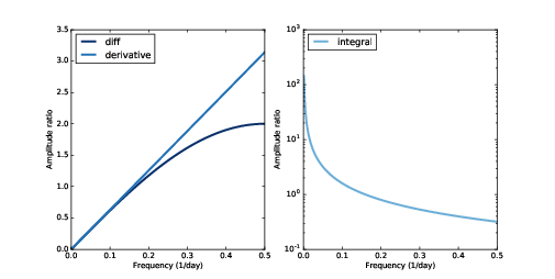
圖9.3 對應到差分與微分操作的濾波器(左),對應積分操作的濾波器(右,log-y scale)
圖9.3 顯示了結果。finite difference window 對應到高通濾波器,它的振幅隨頻率增加,在低頻約為線性,之後大略接近線性。下一節我們會了解原因。
9.3 微分 | Differentiation
我們前一節用的 window 在數值上接近一階導數,所以濾波器的效力近似微分的效力。微分在時間域是對應到頻域的簡單濾波器,我們可以用一點小數學來搞清楚。
假設我們有個複數正弦函數,它的頻率是 :
的一階導數是
我們可以重寫成:
換句話說,對 取導數就等於直接把它乘 ,其為一個複數,長度為 ,角度為 。
我們可以計算對應至微分的濾波器,像這樣:
    deriv_filter = close.make_spectrum()
deriv_filter.hs = PI2 * 1j * deriv_filter.fsclose 的頻譜開始,它有正確的長度與幀率,然後用 取代 hs。圖9.3 (左)顯示這個濾波器,它是個直線。我們在 7.4節看過,複數正弦乘複數會有兩個效果:它的長度相乘,這裡是乘上 ,然後有相位移,在這裡是 。
如果你對算子(operator)與 eigenfunctions 熟悉的話,每個 都是一個微分算子的 eigenfunction,其 eigenvalue 為 ,參見 http://en.wikipedia.org/wiki/Eigenfunction
如果你對這些說法不熟,這裡解說一下:
- 一個算子就是一個函數,只是他的輸入是個函數,輸出也是個函數。例如,微分就是一個算子。
- 有個函數 ,我們說它是一個算子 的 eigenfunction。那就是說,把 用到 身上的效果,等於 乘上某個倍數。也就是寫成這樣: 。
- 在這狀況下,那個倍數 我們叫它 eigenvalue,它對應的 eigenfunction 為 。
- 一個給定的算子也許有許多 eigenfunction,每一個都有其對應的 eigenvalue。
對於多於一個成份的訊號來說,這過程只有難一點點:
- 把訊號表示為數個複數正弦的和
- 用乘法計算出每個成份的導數
- 把每個微分過的成份加起來
Spectrum 提供一個方法可以用濾波器:# class Spectrum:
def differentiate(self):
self.hs *= PI2 * 1j * self.fs deriv_spectrum = close.make_spectrum()
deriv_spectrum.differentiate()
deriv = deriv_spectrum.make_wave()
圖9.4 每日漲跌比較圖。用
np.diff 計算與用 微分濾波器 計算。圖9.4 比較兩個方法計算出的每日漲跌,一個是用
np.diff與剛才計算的導數所計算的。我選序列中前 50 個值,讓我們可以看比較清楚。算出的導數的數值比較雜亂,因為它會增強高頻成份的振幅,如同圖9.3 (左)所示。同時,前幾個導數的元素非常嘈,原因是它是基於 DFT 方法所計算的,而 DFT 有個假設是訊號是週期性的。所以,在計算上有將最後一元素連回第一個元素,因此造成邊界有人為的影響。
總結一下我們提過的:
- 計算訊號中兩個前後值的差,可以表示成一個 window 對訊號做卷積。它的結果會近似一階導數。
- 在時間域的微分對應到頻域是個簡單濾波器。對週期訊號而言,結果即為一階導數。對一些非週期訊號而言,它接近導數。
它對於第十章會提到的線性分析,非時變系統特別有用。
9.4 積分 | Integration

圖9.5 比較原時間序列與積分過的導數
在前一節,我們展示過,在時域的微分會對應頻域的一個簡單濾波器:把每個成份乘上 。因為積分是微分的相反,所以它也對應到一個簡單濾波器:把每個成分除 。
我們可以如此計算這濾波器:
    integ_filter = close.make_spectrum()
integ_filter.hs = 1 / (PI2 * 1j * integ_filter.fs)Spectrum 提供一個方法來應用積分濾波器:# class Spectrum:
def integrate(self):
self.hs /= PI2 * 1j * self.fs integ_spectrum = deriv_spectrum.copy()
integ_spectrum.integrate()NaN,這是浮點數裡特別的值,其為表達「不是一個數」的意思。我們可以特別處理這個問題,在把頻譜轉回波之前把這個值改為零。 integ_spectrum.hs[0] = 0
integ_wave = integ_spectrum.make_wave()如果我們提供這「積分的穩定」為證其結果是相等的,這就確認積分濾波器是正確的微分濾波器的相反。
9.5 累積和 | Cumulative sum

圖9.6 鋸齒波與其頻譜
譯註:把圖的位置從 9.4節搬到這裡
差分操作也近似微分,其累積和近似積分。我用一個鋸齒波訊號來示範。
    signal = thinkdsp.SawtoothSignal(freq=50)
in_wave = signal.make_wave(duration=0.1, framerate=44100)Wave 提供個方法來計算波的累積和之後產生一個新的波:# class Wave:
def cumsum(self):
ys = np.cumsum(self.ys)
ts = self.ts.copy()
return Wave(ys, ts, self.framerate)in_wave 的累積和: out_wave = in_wave.cumsum()
out_wave.unbias()
圖9.7 拋物線波與其頻譜
圖9.7 顯示它的波形與頻譜。如果你在第二章有做練習,這個波形應該會熟悉,它是拋物線訊號。
把拋物波的頻譜與鋸齒波的頻譜比較,前者的振幅下降非常快。在第二章在,我們看過鋸齒波下降正比於 。因為累積和接近積分,積分濾波器成份正比於 ,所以拋物波下降正比於 。
我們可以計算其對應到累積和的濾波器,把結果視覺化:
    cumsum_filter = diff_filter.copy()
cumsum_filter.hs = 1 / cumsum_filter.hscumsum 是 diff 的反操作,我們從 diff_filter 的複製開始,其為對應 diff 的操作,然後把 hs 反向。
圖9.8:對應到累積和與積分的濾波器
圖9.8 顯示累積和與積分的濾波器。累積和是個很好的積分近似,除了在高頻部份下降有點快。
為了要確認這是正確的累積和的濾波器,我們可以比較
out_wave 頻譜與 in_wave 頻譜的比例: in_spectrum = in_wave.make_spectrum()
out_spectrum = out_wave.make_spectrum()
ratio_spectrum = out_spectrum.ratio(in_spectrum, thresh=1)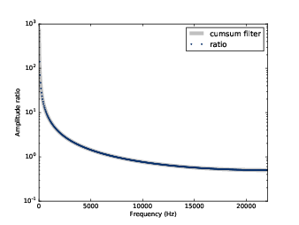
圖9.9:對應累積和的濾波器與應用前後之頻譜的實際比例
以下是計算比例的方法:
    def ratio(self, denom, thresh=1):
        ratio_spectrum = self.copy()
        ratio_spectrum.hs /= denom.hs
        ratio_spectrum.hs[denom.amps < thresh] = np.nan
return ratio_spectrumdenom.amps 小的時候,結果的比例是雜亂的,所以我把這些值設成 NaN。圖9.9 顯示其比例與對應累積和的濾波器。其證明
diff 的濾波器的反轉會得到 cumsum 的濾波器。最後,我們可以證明卷積理論,在頻域上應用
cumsum 濾波器: out_wave2 = (in_spectrum * cumsum_filter).make_wave()out_wave2 等同於 out_wave,而前者是我們用 cumsum 算出來的。所以卷積理論可用!但要注意這個示範只適用於週期訊號。9.6 積分噪音 | Integrating noise
在 4.3節,我們產生布朗噪音,方法是計算白噪音的累積和。現在我們了解cumsum 在頻域上的效應,我們可以進一步看看布朗噪音的頻譜。白噪音是平均地在所有頻率有相同功率。當我們計算累積和,每個成分的振幅會除以 。因為功率是振幅的平方,所以每個成份的功率就除以 。所以平均來說,在頻率 的功率會正阰於 :
此處 是常數而且不重要。接下來兩邊取 log 後得到:
這就是為什麼當我們在 log-log scale 畫出布朗噪音時,會預期得到一個斜率為(或接近) -2 的直線。
在 9.1節,我們畫臉書收盤價的頻譜,估算其斜率為 -1.9,約與布朗噪音的一致。許多股票都有相同的頻譜。
當我們使用
diff 算子來計算每日變化,我們會把每個成份的振幅乘上正比於 的濾波器,這代表我們把每個成分的功率都乘上 。這項操作在 log-log scale 的功率頻譜上加了個 2 的斜率,這就是為什麼結果的斜率估算為 0.1 (還是低一點,因為 diff 只是近似微分)。9.7 練習
Solutions to these exercises are in chap09soln.ipynb.Exercise 1 The notebook for this chapter is
chap09.ipynb. Read through it and run the code.In Section 9.5, I mentioned that some of the examples don’t work with non-periodic signals. Try replacing the sawtooth wave, which is periodic, with the Facebook data, which is not, and see what goes wrong.
Exercise 2 The goal of this exercise is to explore the effect of
diff and differentiate on a signal. Create a triangle wave and plot it. Apply diff and plot the result. Compute the spectrum of the triangle wave, apply differentiate, and plot the result. Convert the spectrum back to a wave and plot it. Are there differences between the effect of diff and differentiate for this wave?Exercise 3 The goal of this exercise is to explore the effect of
cumsum and integrate on a signal. Create a square wave and plot it. Apply cumsum and plot the result. Compute the spectrum of the square wave, apply integrate, and plot the result. Convert the spectrum back to a wave and plot it. Are there differences between the effect of cumsum and integrate for this wave?Exercise 4 The goal of this exercise is the explore the effect of integrating twice. Create a sawtooth wave, compute its spectrum, then apply
integrate twice. Plot the resulting wave and its spectrum. What is the mathematical form of the wave? Why does it resemble a sinusoid?Exercise 5 The goal of this exercise is to explore the effect of the 2nd difference and 2nd derivative. Create a
CubicSignal, which is defined in thinkdsp. Compute the second difference by applying diff twice. What does the result look like? Compute the second derivative by applying differentiate to the spectrum twice. Does the result look the same?Plot the filters that correspond to the 2nd difference and the 2nd derivative and compare them. Hint: In order to get the filters on the same scale, use a wave with frame rate 1.


沒有留言:
張貼留言